Okay! You have your data read into R, you’ve looked at it a little bit with plots and other descriptive statistics. Now, it’s time to run some tests! Do some more rigorous examinations and comparisons. For a detailed description of any of the tests and calculations I show here, you should look elsewhere (Wikipedia is actually a good source!). I am only going to show you how to do them in R and how to interpret the results.

There are so many statistical tests out there in the wild and each do many fantastic and complex things! It’s hard to know where to start or where to define the basics. For me the basics are comparing one or two sets of information. In another post, we will go over tests that compare three or more groups.

Again, for these examples, I will use the mtcars data set that is installed along with R. Note, that in order to get access to just a single column or variable in data sets in R you use the $ symbol. For example, to get only the values of the mpg variable from the mtcars data set, use the code mtcars$mpg.

Correlations

Correlations show the relationship between two variables. There are three options here: positive (one goes up, the other goes up), negative (one goes up, the other goes down), and none.

To get a correlation in R, use the cor() function. This function requires two arguments, the two variables you want to compare. It also helps to create a scatterplot so you can visualize what is going on. In this example, while not a perfect line, there appears to be a negative relationship between a car’s miles per gallon and its horsepower. So as the horsepower increases, the miles per gallon decreases.

cor(mtcars$hp, mtcars$mpg)

## [1] -0.7761684

plot(mtcars$hp, mtcars$mpg)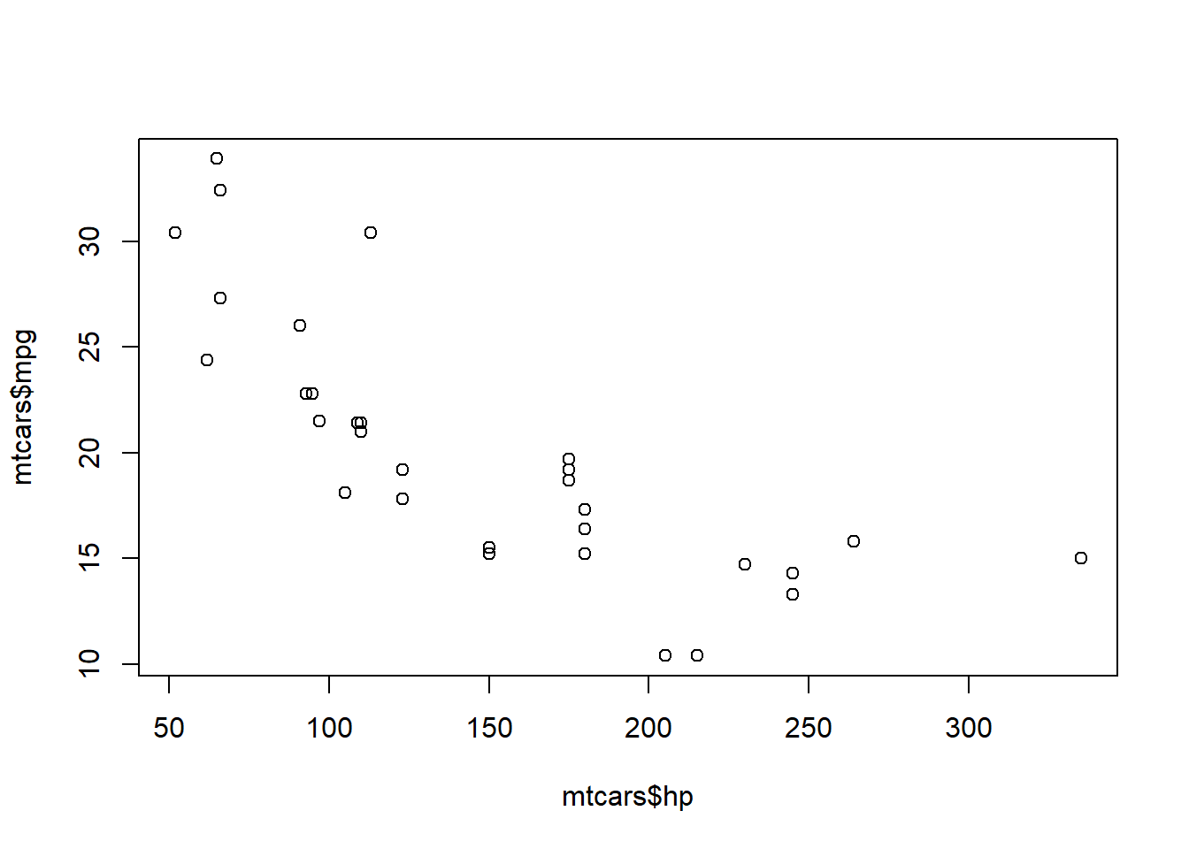

Comparing the Mean

There are multiple ways to test whether the mean of a variable is equal to a certain value or is similar to the mean of a second variable. I’ll go over the ones you will see most often.

One Sample $t$-Tests

The tests you will see most often are t-tests. One sample t-tests compare the mean of one variable to a value (most often zero). Let’s compare and see if the average miles per gallon is significantly different from zero.

t.test(mtcars$mpg, mu = 0)

## 
##  One Sample t-test
## 
## data:  mtcars$mpg
## t = 18.857, df = 31, p-value < 2.2e-16
## alternative hypothesis: true mean is not equal to 0
## 95 percent confidence interval:
##  17.91768 22.26357
## sample estimates:
## mean of x 
##  20.09062

There is a lot of output that appears here, but if you go through it piece by piece, it becomes clear. First, the test statistic, degrees of freedom, and p-value will be the numbers you report in a written report. Here, the interpretation would be “The average miles per gallon of the examined vehicles is $20.09$, which is significantly different from zero ($t(31)=18.86$, $p<.001$).”

Two Sample $t$-Tests

There are two different kinds of two sample t-tests: Independent and Dependent (or Paired). However, the code needed is very similar to the previous command, with a few additions. For independent tests, add in the second variable. For dependent variables, you need the extra argument paired = TRUE so R knows that the groups are connected.

# Independent
t.test(mtcars$mpg, mtcars$hp)

#Dependent
t.test(mtcars$mpg, mtcars$hp, paired = TRUE)

The output and interpretations will also be similar. Instead of being different from a specific value, discuss how the groups are different from one another: “The average miles per gallon of the examined vehicles is $20.09$, which is significantly lower than the average horsepower of the vehicles ($t(31.48)=-10.41$, $p<.001$).” These results are expected since these are actually measuring two very different things. In real tests, the observed variable should be the same for both groups. The set up for the code would be a little different as we need to define the groups to compare.

# We will use the variable for automatic transmission
# 0 = automatic, 1 = manual
mtcars$am <- as.factor(mtcars$am)

# Independent
t.test(mpg ~ am, data = mtcars)

Non-parametric Tests

The final example I have for comparing the means is the Non-parametric tests. You can use these tests in place of a t-test, especially when the doesn’t follow a known distribution. The test to compare means is called the Wilcoxon Ranked Sum test. It is based on the “sign” and “rank” of a data point, hence the name Rank Sum. Non-parametric tests are interpreted in a similar way to t-tests and the code again is very similar.

# Independent
wilcox.test(mtcars$mpg, mtcars$hp)
# OR
wilcox.test(mpg ~ am, data = mtcars)

#Dependent
wilcox.test(mtcars$mpg, mtcars$hp, paired = TRUE)

So far we have gone over basic statistics, plotting, importing data, and started reviewing some basic statistical tests. We will finish the discussion of statistical tests next!

R Basics: Statistical Tests Part 1

Correlations

Comparing the Mean

One Sample \(t\)-Tests

Two Sample \(t\)-Tests

Non-parametric Tests