ANOVAs

The most common way to compare three or more group averages is by conducting an Analysis of Variance, or ANOVA. The important thing to know about ANOVAs is that it will compare any number of groups, however it will only tell you that a difference exists SOMEWHERE. It doesn’t tell you which groups are different. Post-hoc (or after-the-fact)tests often follow an ANOVA test to determine where the difference is located.

In my example, I adjusted the data set a little by making one of the variables a factor variable. This will define the groups to use in the ANOVA test.

mtcars$cyl <- as.factor(mtcars$cyl)

anova <- aov(mpg ~ cyl, data = mtcars)

summary(anova)

To get the results of the ANOVA from R, you need to ask for a summary of the ANOVA model. The last two columns of the table that appears hold the test statistic and the p-value for the ANOVA. R is really nice here because it will star the significant results in this table. To interpret this result, you would say something like “There is a difference in the average miles per gallon in cars with different numbers of cylinders in the engine (\(F(2,29)=39.7\),\(p<.001\)).”.

In this example, I have done a one-way ANOVA. The “one” refers to the one factor I used to define my groups. If I had second factor in the data set, I would perform a two-way ANOVA. The code would be similar to above, but you would add the second factor to the ANOVA model statement.

Regression

Regression is a vast area of statistics. I could write an entire blog about regression. However, here I’ll go over the basics of conducting a simple regression in R. Regression is another way to examine the relationship between variables. Using this method, you can see an estimation of how much a change in one variable can effect another.

The variables in regression are often divided into what you are trying to predict (the dependent variable) and what you are using to make the prediction (the independent variables or predictors). It’s important to make this distinction before you start! For our example, let’s predict miles per gallon from horsepower.

fit <- lm(mpg ~ hp, data=mtcars)
summary(fit)

## 
## Call:
## lm(formula = mpg ~ hp, data = mtcars)
## 
## Residuals:
##     Min      1Q  Median      3Q     Max 
## -5.7121 -2.1122 -0.8854  1.5819  8.2360 
## 
## Coefficients:
##             Estimate Std. Error t value Pr(>|t|)    
## (Intercept) 30.09886    1.63392  18.421  < 2e-16 ***
## hp          -0.06823    0.01012  -6.742 1.79e-07 ***
## ---
## Signif. codes:  0 '***' 0.001 '**' 0.01 '*' 0.05 '.' 0.1 ' ' 1
## 
## Residual standard error: 3.863 on 30 degrees of freedom
## Multiple R-squared:  0.6024, Adjusted R-squared:  0.5892 
## F-statistic: 45.46 on 1 and 30 DF,  p-value: 1.788e-07

The first thing you should not is how similar this output is to ANOVA output. When you predictor variable is categorical, or defines a group, regression and ANOVA should be pretty similar. The second thing you should look at is the plot of the regression line.

plot(mtcars$hp, mtcars$mpg)
abline(fit)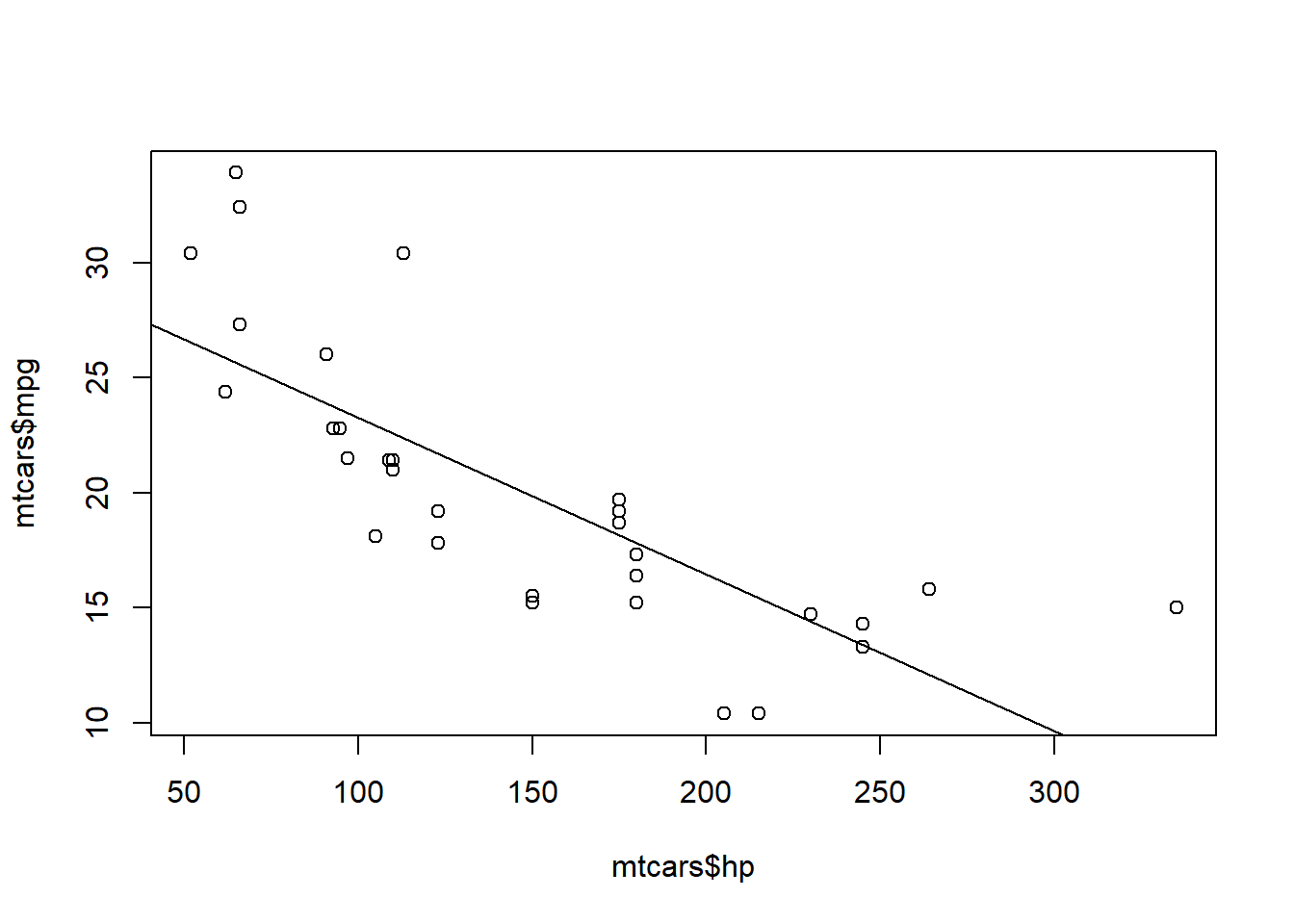

It’s the same plot that we had when we looked at the correlation between these two variables. We have just added the regression line to gain some more insight into the relationship between horsepower and correlation.

Tests of Independence

The last tests I will go over as basics are the Chi-Squared (\(\chi^2\)) test and Fisher’s Exact test. These tests are applied when you are classifying data into multiple groups. Is there a difference between the number of observations who fall into each group?

Since these tests rely on frequencies of observations in a specific category, it is helpful to create a frequency table.

# Number of cylinders in engine
mtcars$cyl <- as.factor(mtcars$cyl)

# Automatic transmission (0 = automatic, 1 = manual)
mtcars$am <- as.factor(mtcars$am)

freq <- table(mtcars$am, mtcars$cyl)
freq

##    
##      4  6  8
##   0  3  4 12
##   1  8  3  2

A Chi-Squared (\(\chi^2\)) test or Fisher’s Exact test will test if the differences in the amount in each group is significant. The difference between the tests is that, as the name implies, a Fisher’s test is more exact. However, the output from the Fisher’s test in R only includes the p-value, so I would recommend using and reporting the Chi-squared value instead.

chisq.test(freq)

## Warning in chisq.test(freq): Chi-squared approximation may be incorrect

## 
##  Pearson's Chi-squared test
## 
## data:  freq
## X-squared = 8.7407, df = 2, p-value = 0.01265

#fisher.test(freq)

The output would be interpreted as: “The frequency of cars in each group is different from what was expected (\(\chi^2(2)=8.74\), \(p=.013\)).”